
Introduction and Background
Vehicle trajectory prediction, which aims to forecast future positions and movement of vehicles based on historical data and surrounding environment information, is essential in advanced driver assistance systems (ADAS) and autonomous vehicles (AV) [1]. This project focuses on analyzing the performance of Gaussian Mixture Model (GMM), linear/logistic regression, and Long Short-Term Memory (LSTM) methods to predict vehicle trajectories for autonomous driving.
In recent years, machine learning techniques have been employed to handle the complexities of different driving patterns and dynamic traffic conditions. One study which examined LSTM, Gated Recurrent Units (GRU), and Stacked Autoencoders (SAEs) models has shown that LSTM performed better with a MAE of 6.78 [2]. Further exploration of LSTM models includes an addition of spatiotemporal attention (STA) to explain how historical vehicle trajectories (temporal-level attention) and neighboring vehicles (spatial-level attention) help explain vehicle trajectory [3]. There are opportunities to explore the incorporation of contextual information such as road layouts and relative trajectory prediction of surrounding vehicles to enhance trajectory prediction [4].
The Next Generation Simulation (NGSIM) dataset will be used for this project, which contains vehicle trajectory data across Atlanta, Los Angeles, and Emeryville. This time-series dataset includes vehicle-specific information such as vehicle ID, time stamps, and position data (both global and local coordinates), along with features like velocity, acceleration, vehicle length, and class.
Problem Definition
The problem we aim to solve is the prediction of future positions and movement of vehicles based on historical and surrounding environment information using machine learning. This can enhance safety of ADAS through improved collision warning systems for drivers and enhance AV’s ability to make decisions that ensure safety. Challenges in vehicle trajectory prediction include complex interactions of vehicles and dynamic traffic conditions; and noise in data attributed by sensor errors due to building obstructions [4]. Our project analyzes the effects of these machine learning algorithms in the problem of autonomous driving trajectory prediction by implementing GMM, linear/logistic regression, and LSTM.
Method
Data Preprocessing
 | 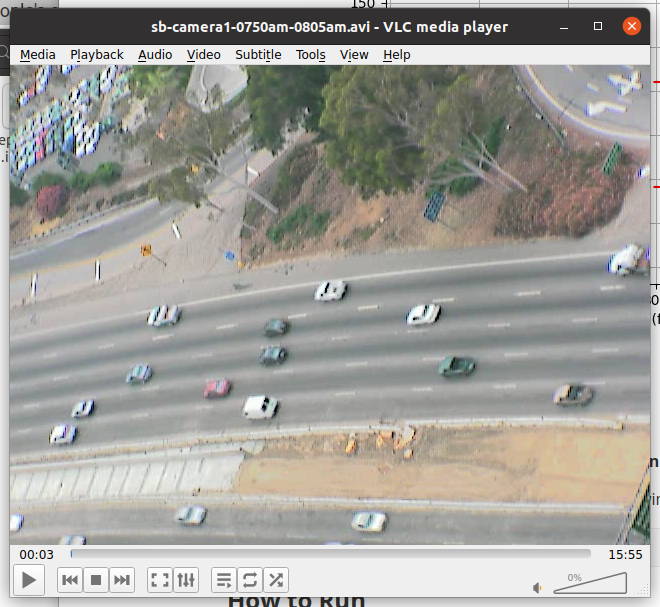 |
Figure 1: Data visualization and actual scenario of US101 highway
 | 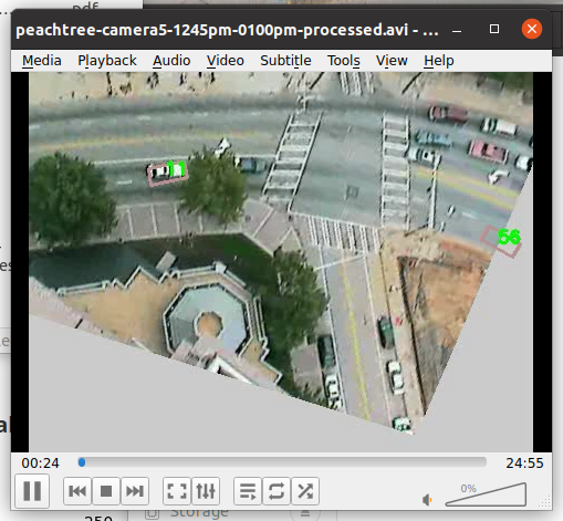 |
Figure 2: Data visualization and actual scenario of Peachtree street
In the preprocessing stage, we implemented data cleaning, feature engineering, and regularization to prepare the data for analysis. To optimize efficiency, we processed the US101 highway, I80 street, and Peachtree street datasets in parallel using a combination of threads and processes, ensuring faster and more effective data handling across multiple datasets simultaneously. Using data cleaning to remove missing or anomalous values, which may arise from sensor errors or incomplete vehicle records. Feature engineering will also be applied to create new attributes, such as the relative velocity between vehicles and lane change indicators, critical for modeling complex vehicle behavior. Finally, we split the data sets for each different scenario into 70% training set, 10% validation set, and 20% test set.
| Left Lane | Same Lane | Right Lane |
|---|---|---|
| Cell 0 | Cell 13 | Cell 26 |
| Cell 1 | Cell 14 | Cell 27 |
| ... | ... | ... |
| Cell 6 | Ego | Cell 32 |
| ... | ... | ... |
| Cell 12 | Cell 25 | Cell 38 |
Table 1: An example layout of grid neighbors around an ego vehicle located at the center.
Considering the interactive environment when the vehicle is driving, we obtain the vehicle's neighbors as one of the new features created by feature engineering. We obtain the IDs of the ego's neighbor vehicles and store them in a 3x13 matix (Grid_Neighbor). assigns neighboring vehicle IDs to a grid based on their relative position to the ego vehicle, using vertical (and, at intersections, horizontal) offsets to determine each vehicle's grid index. By calculating these indices, it places each neighbor in the appropriate grid cell in relation to the ego vehicle’s lane and position. Due to the US101 dataset does not contain the feature of the vehicle’s turning direction, we also reconstruct this feature specifically for the US101 data. We check if the vehicle is maintaining its lane, turning left, or turning right based on the vehicle’s lateral (lane) position over a time window of 4 seconds in the past and 4 seconds in the future. In addition, in order to enable the model to better learn the lateral distance, we also added yaw angle as a new feature. The data after feature engineering is shown in Table 2.
| Data | Description |
|---|---|
| Vehicle_ID | Vehicle identification number |
| Frame_ID | Frame Identification number |
| Global_Time | Elapsed time in milliseconds since Jan 1, 1970 |
| Local_X | Lateral (X) coordinate of the front center of the vehicle in feet with respect to the left-most edge of the section in the direction of travel |
| Local_Y | Longitudinal (Y) coordinate of the front center of the vehicle in feet with respect to the entry edge of the section in the direction of travel |
| v_length | Length of vehicle in feet |
| v_Width | Width of vehicle in feet |
| v_Class | Vehicle type: 1 - motorcycle, 2 - auto, 3 - truck |
| v_Vel | Instantaneous velocity of vehicle in feet/second |
| v_Acc | Instantaneous acceleration of vehicle in feet/second square |
| Lane_ID | Current lane position of vehicle |
| Int_ID | Intersection in which the vehicle is traveling |
| Section_ID | Section in which the vehicle is traveling |
| Direction | Moving direction of the vehicle. 1 - east-bound (EB), 2 - north-bound (NB), 3 - west-bound (WB), 4 - south-bound (SB) |
| Movement | Movement of the vehicle. 1 - through (TH), 2 - left-turn (LT), 3 - right-turn (RT) |
| Grid_Neighbors | The neighbors of ego at the same frame |
| Space_Headway | Spacing provides the distance between the frontcenter of a vehicle to the front-center of the preceding vehicle |
| Time_Headway | Time Headway provides the time to travel from the front-center of a vehicle (at the speed of the vehicle) to the front-center of the preceding vehicle |
| Location | Name of street or freeway |
| Theta | The yaw of vehicle |
Table 2: Data structure after feature processing (including the data necessary for data visualization, such as the length and width of the vehicle).
Data Analysis
|
|
|
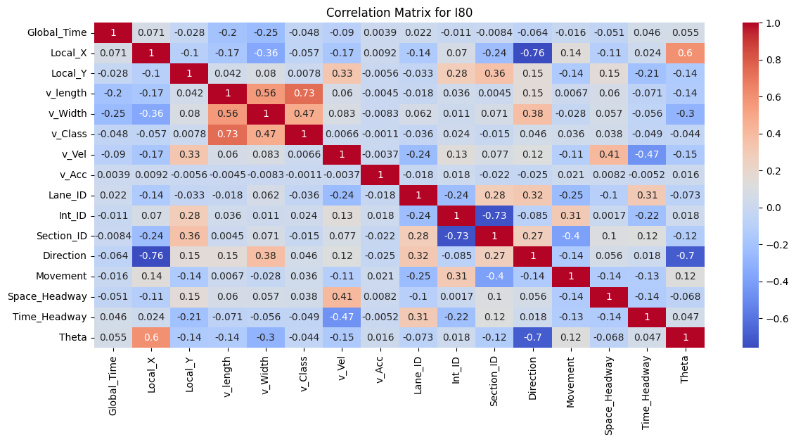
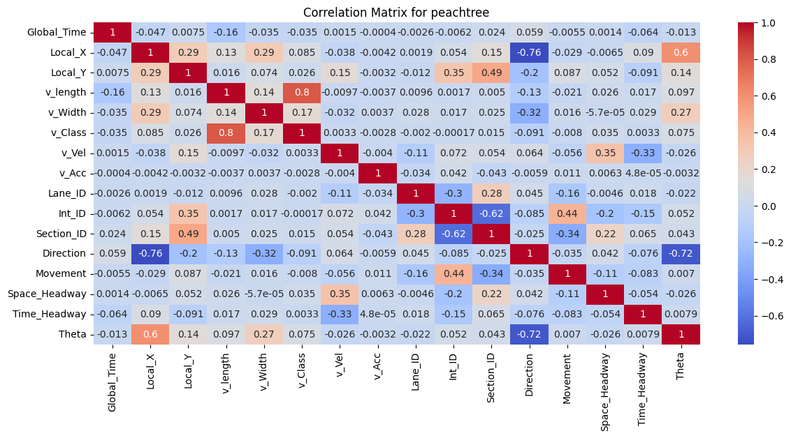
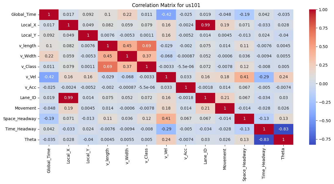
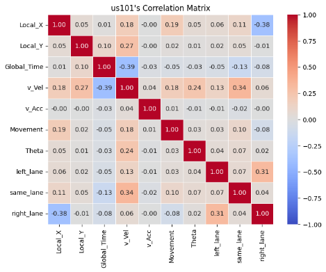
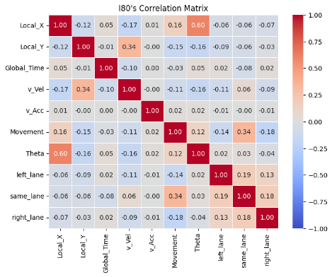
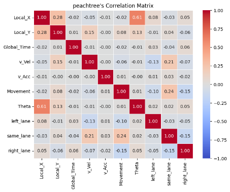
Figure 3: Correlation Matrix for I80, Peachtree Street, and US101
To better understand the data, the correlation between features was examined. As shown in the correlation matrices, for all I80, Peachtree Street, and US 101 datasets, the vehicle length, vehicle width and vehicle class are highly correlated as vehicle class (motorcycle, auto, or truck) is associated with the size of the vehicle. In addition, theta is positively correlated with Local_X for both the I80 and Peachtree Street data, suggesting that theta could be a good feature to explore during model implementation to predict vehicle position.
|
|
|
|
|
|
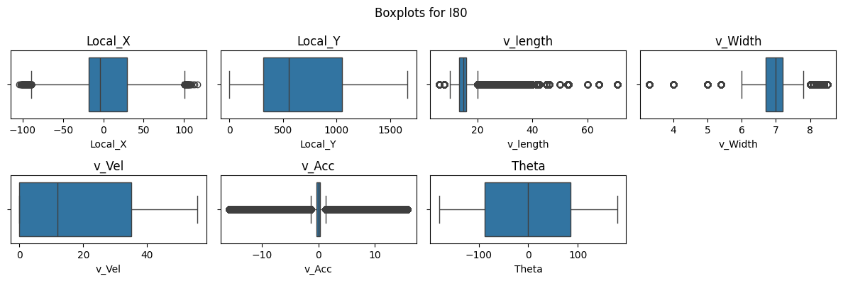
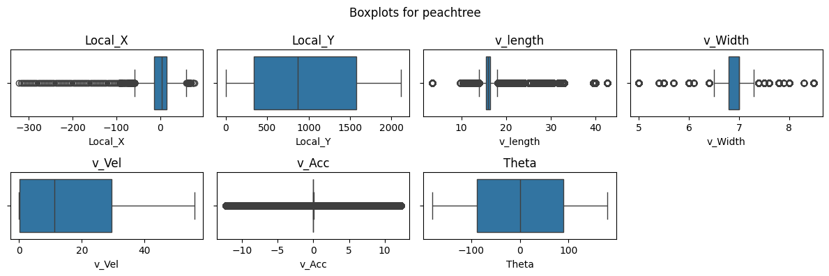
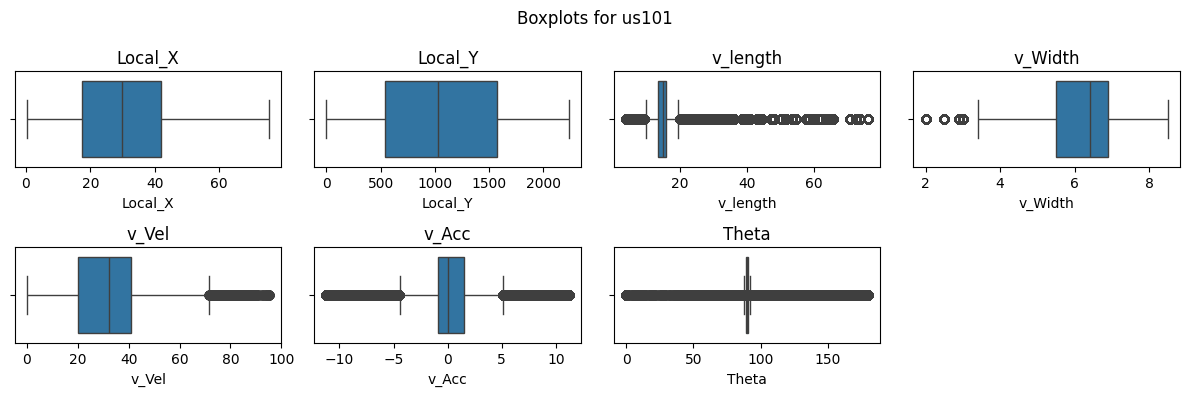
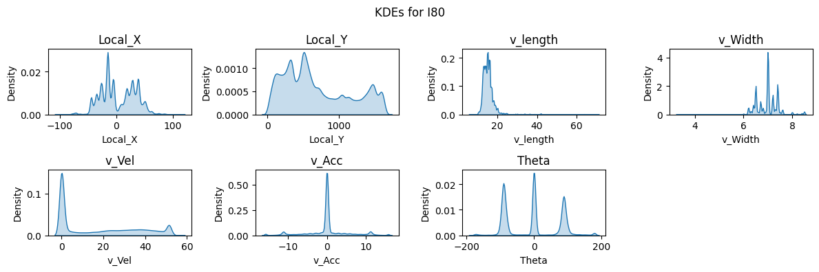
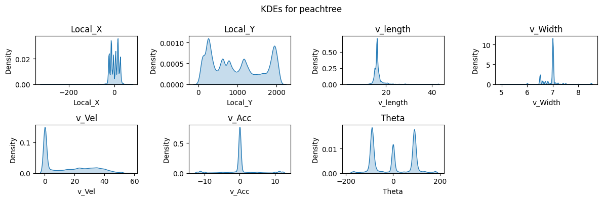
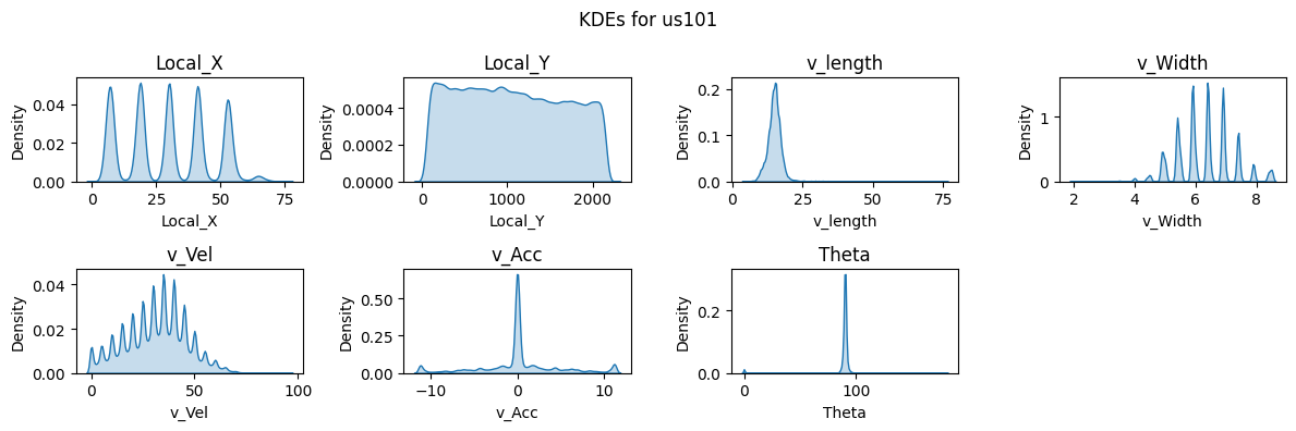
Figure 4: Boxplots and KDEs for I80, Peachtree Street, and US101.
Boxplots and kernel density estimate (KDE) plots were created for a subset of key features to visualize the distribution of the dataset. These plots show that Local_X, Local_Y, and Vehicle Velocity have a wider distribution in values. Given the multiple intersections for I80 and Peachtree Street, theta is multimodal and there are more timeframes where vehicles are stationary as shown in the density plots. Overall, the distribution of data for I80 and Peachtree Street are more similar as compared to US101 as I80 and Peachtree Street are local roads while US101 is a highway.
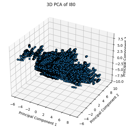
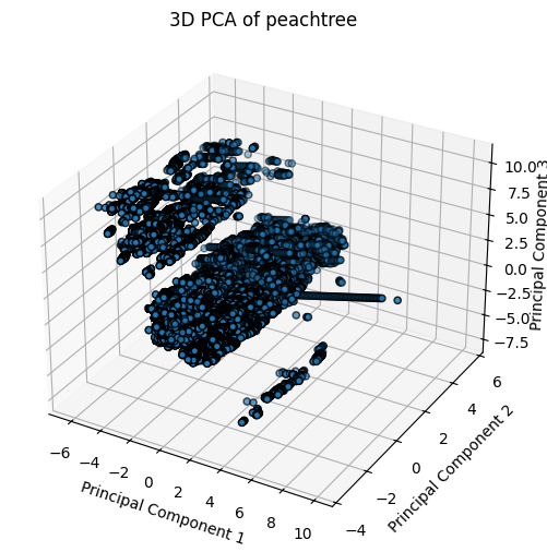
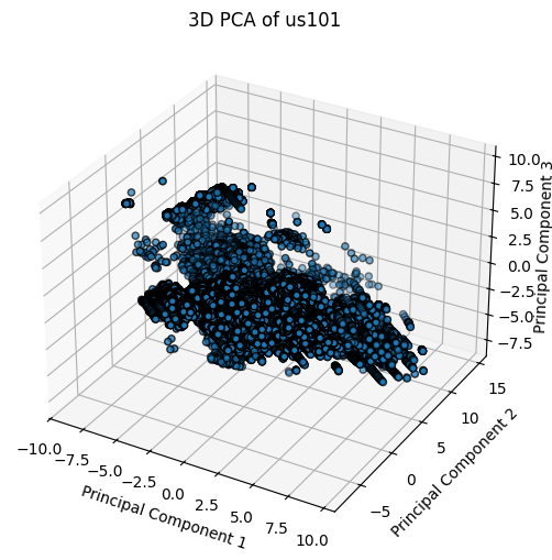
In addition to visualizing the data using boxplots and KDEs, Principal Component Analysis (PCA) was used to visualize, explore, and understand the data.
|
|
|
Figure 5: 3D PCA Plots for I80, Peachtree Street, and US101.
|
|
|
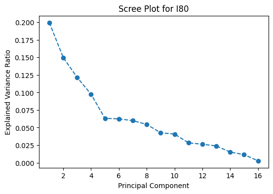
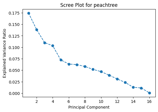
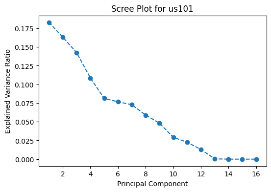
Figure 6: Scree Plots for I80, Peachtree Street, and US101.
|
|
|
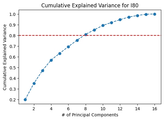
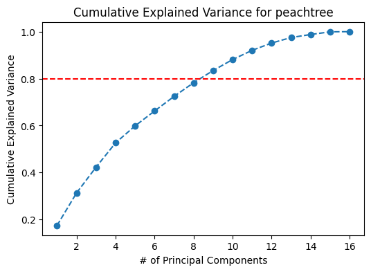
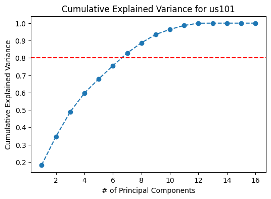
Figure 7: Cumulative Variance Plots for I80, Peachtree Street, and US101.
Based on the scree plots in Figure 6, the optimal number of principal components to select is five. The top five principal components result in about 60-65% of the variance explained. However, if a higher proportion of variance from the data is to be retained, for example 80%, the top 8 principal components would have to be considered.
|
|
|
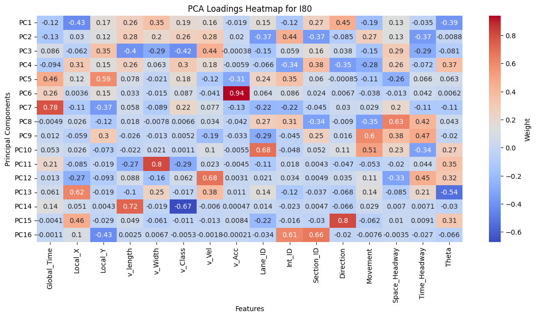
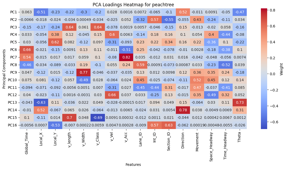
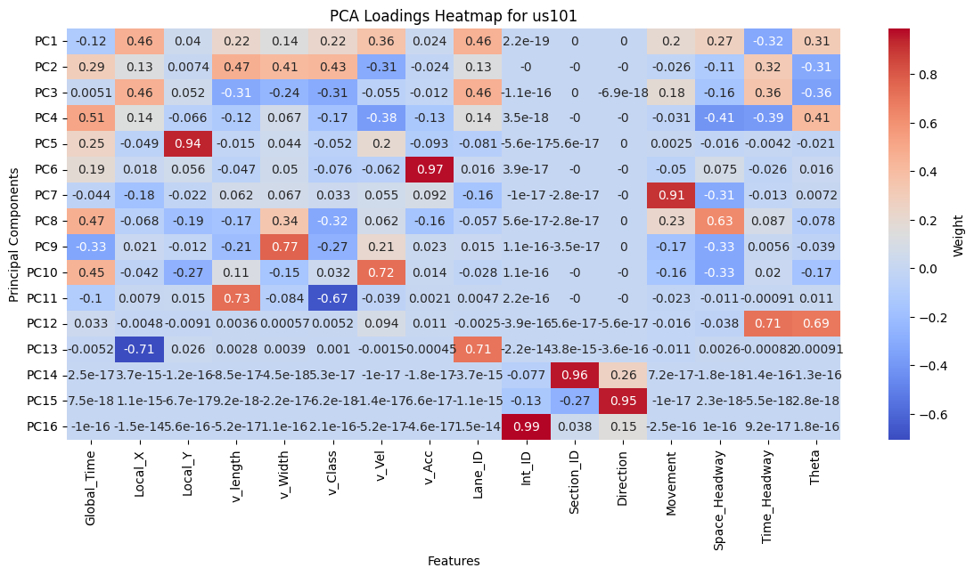
Figure 8: PCA Loadings for I80, Peachtree Street, and US101.
The PCA loadings heatmap shows the combination of features that contribute to each principal component. Examining the top 5 principal components provide insight into key drivers of variance in the data which include: Local_X, Local_Y, Vehicle Length, Velocity, Lane ID, and Theta. While Direction, Intersection ID, and Section ID contribute to the top principal components for I80 and Peachtree, it does not for US101 because US101 is a highway with minimal lateral deviation, while I80 and Peachtree have intersection-rich road layouts. Further exploration using these principal components can be evaluated during model implementation.
Method Implemented
LSTM
The TrajectoryNetwork model based on LSTM has been designed for predicting the ego of future trajectories. The TrajectoryNetwork model utilizes structured historical and future sequences for both the ego vehicle and its neighboring vehicles to inform trajectory predictions. For each vehicle, a sequence of past states is extracted, starting from the current timestamp and moving backward across a predefined window of historical data. This sequence includes the vehicle's recent spatial positions, speed, acceleration, heading direction, and movement type, forming a comprehensive view of its recent trajectory. This historical sequence is crucial, as it provides temporal patterns that inform the vehicle’s current motion trends. Additionally, for each neighboring vehicle within a defined spatial grid around the ego vehicle, a corresponding history is collected. This grid-based approach allows the model to capture interactions and relationships between the ego vehicle and its immediate traffic environment, adding a layer of social context to the input data.
Future states are also gathered to serve as the ground truth target for the model during training. These future sequences, spanning a specified prediction horizon, contain the actual observed positions of the ego vehicle for upcoming time steps. By framing these future trajectories as the training targets, the model learns to minimize the discrepancy between its predictions and actual observed data. The use of a masked loss function during training allows the model to handle sequences of varying lengths across vehicles. This combination of historical encoding for both ego and neighbor vehicles, along with the future trajectory as a training objective, allows the TrajectoryNetwork to effectively model complex interactions within the traffic environment and produce robust, accurate predictions of the ego vehicle’s future path.
Linear Regression
On a straight road, a vehicle typically moves with constant velocity, and the position can be represented by a simple linear equation. For example, if the vehicle moves with a constant speed, its position at time t can be described as a linear function of time, making linear regression an ideal choice for such cases.
The attribute “Grid_Neighbours” represents the neighbouring cars on the left, same and right lane. Its row_index corresponds to the relative distance to the current vehicle. To feed into the Linear Regression model, this attribute is expanded to left_lane, same_lane and right_lane attributes, where the value represents the relative distance from the current vehicle. If none are present, the value is –1.
The ground truth y value would be the 10 (x, y) coordinates of the current vehicle from lag=1 ... 10 frames later. Linear Regression from scikit-learn is hence implemented on the curated training data to form the baseline model comparison.
Gaussian Mixture Model
The Gaussian Mixture Model (GMM) approach has been implemented to capture the probabilistic nature of vehicle trajectories. Unlike deterministic approaches, GMM can model the uncertainty in vehicle movements, particularly important at intersections and complex traffic scenarios. The model takes into account both the historical trajectory data and the surrounding vehicle context.
The feature set combines vehicle dynamics (position, velocity, acceleration) with contextual information from the Grid_Neighbours structure. Similar to the Linear Regression implementation, the Grid_Neighbours attribute is transformed into left_lane, same_lane, and right_lane features representing relative distances to neighboring vehicles. This spatial awareness helps the model understand the traffic context and potential interaction patterns.
For each prediction step (1 to 10 frames ahead), a separate GMM is trained to capture the distribution of possible future positions. The number of Gaussian components is determined through cross-validation, allowing the model to adapt to different levels of trajectory complexity. This multi-modal approach is particularly valuable in scenarios where multiple plausible future trajectories exist, such as at intersections where a vehicle might turn left, right, or continue straight.
The model outputs probabilistic predictions, providing both the expected trajectory and associated uncertainty estimates. This uncertainty quantification is valuable for downstream applications in autonomous driving systems, where understanding prediction confidence is crucial for safe decision-making.
Result and Discussion
LSTM Result and Analysis
Figure 9: Comparison of LSTM prediction and ground truth in US101 highway
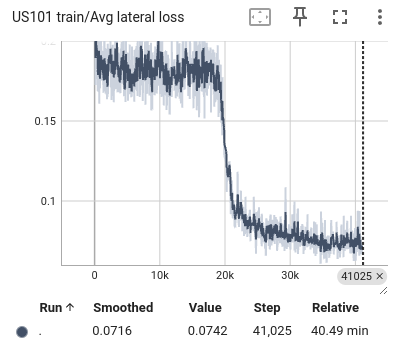
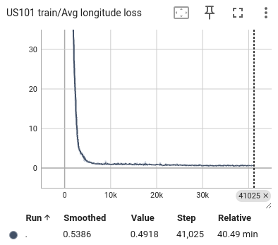
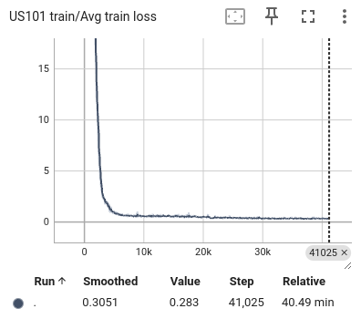
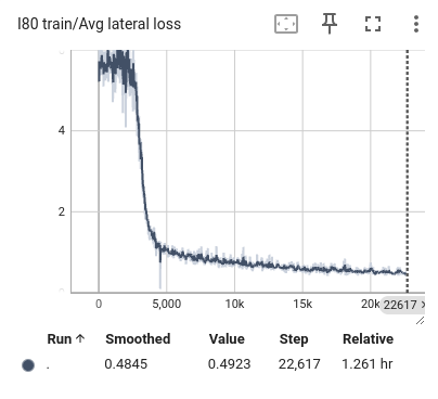
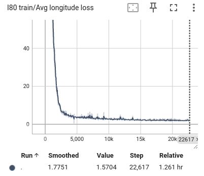
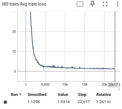
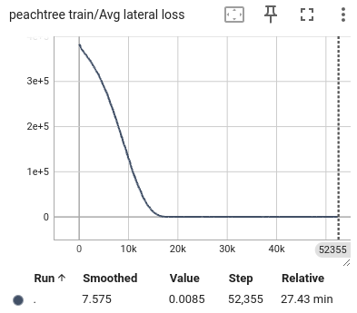
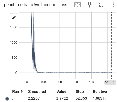
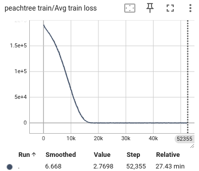
During the training process, we selected the state in the past 1 second as input and predicted all trajectory points in the next 1 second. We also visualized the lateral error loss, longitudinal error loss, and overall error loss of the car, as shown in Figure 9. Overall, the entire training process showed convergence. The initial lateral loss observed in the US101 dataset is comparatively low, whereas the lateral loss for the I80 dataset—and especially for Peachtree Street—is significantly higher. This discrepancy can be attributed to the nature of the road layouts: US101 is predominantly a straight highway with minimal lateral deviation, while I80 includes several intersections, introducing more lateral movement. Peachtree Street, characterized by frequent intersections, exhibits the highest lateral loss due to increased lateral maneuvers required for navigation. Compared to longitudinal information, such as speed and acceleration, the availability of lateral information is considerably more limited. This constraint results in a hierarchy of prediction accuracy across datasets, with US101 demonstrating the highest accuracy, followed by I80, and finally Peachtree Street. This ordering aligns with the structural differences among these road environments, where US101's linearity supports more straightforward predictions compared to the more complex, intersection-rich layouts of I80 and Peachtree Street.
|
|
|
Figure 10: The average loss of US101 training. From left to right are the loss of lateral, longitudinal, and total.
|
|
|
Figure 11: The average loss of I80 training. From left to right are the loss of lateral, longitudinal, and total.
|
|
|
Figure 12: The average loss of peachtree. From left to right are the loss of lateral, longitudinal, and total.
Linear Regression Result and Analysis
|
|
|
Figure 13: Correlation between features
Correlation between features is visualized to identify collinearity as an assumption of linear regression is independence between features. As observed, correlation is mostly low for most features. Some experiments using PCA worsen performance as well, showing preservation of information is key.
|
|
|
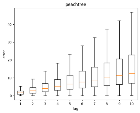
Figure 14: Distance error against lag time
Figure 14 above shows the distribution of errors across lag duration for each dataset. Errors is defined as the euclidean distance between the predicted coordinate and ground truth coordinate. As expected, the further into the future the prediction is, the higher the variance of errors for all datasets. The variance is even higher for I80 and Peachtree as they deal with intersections.
GMM Result and Analysis
|
|
|
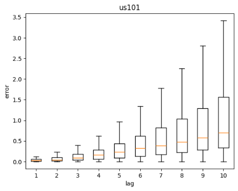
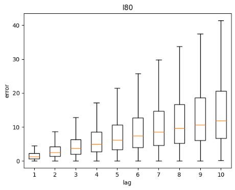
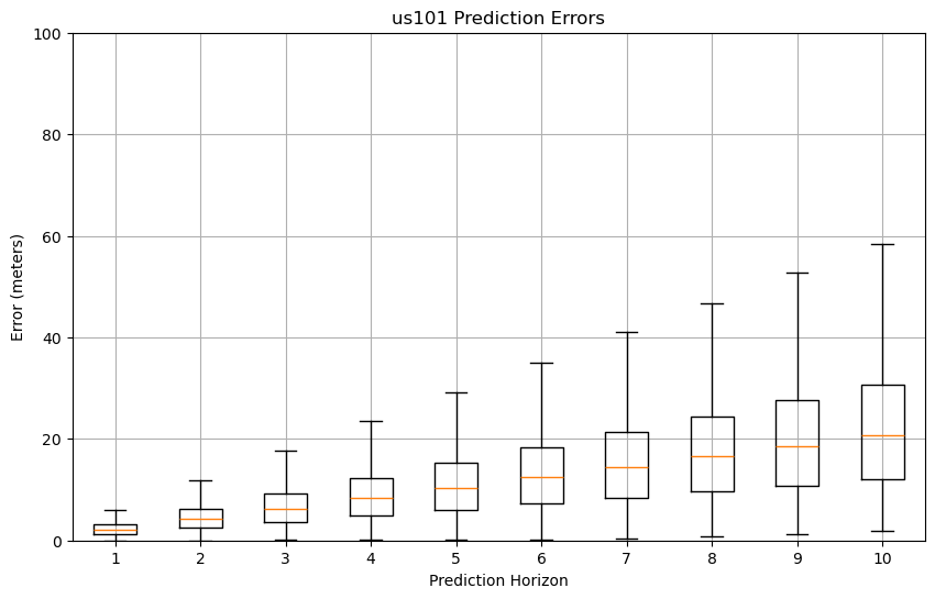
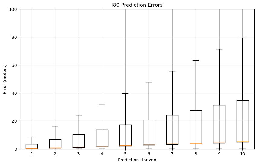
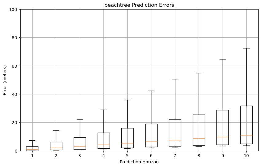
Figure 15: GMM prediction error box plots
Based on the GMM prediction error box plots across three datasets (US101, I80, and Peachtree), the visualization reveals consistent patterns of increasing error magnitude and variance as the prediction horizon extends from 1 to 10 steps. The highway scenario (US101) demonstrates the most stable error progression, with median errors starting at 2-3 meters for step 1 and gradually increasing to 15-20 meters by step 10, while maintaining relatively compact box plots indicating consistent predictions.
In contrast, both I80 and Peachtree datasets, which involve intersections and more complex road configurations, exhibit larger error variances and more extreme outliers, particularly beyond the 7-step prediction horizon, with maximum errors reaching approximately 80 meters at step 10. This pattern suggests that while GMM can maintain reasonable accuracy for short-term predictions (steps 1-3) across all scenarios, its performance significantly deteriorates in complex road environments and longer prediction horizons, highlighting the challenge of maintaining prediction accuracy in diverse traffic conditions and extended time horizons.
|
|
|
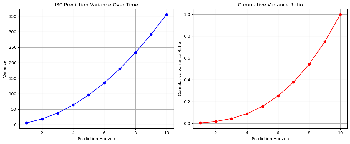
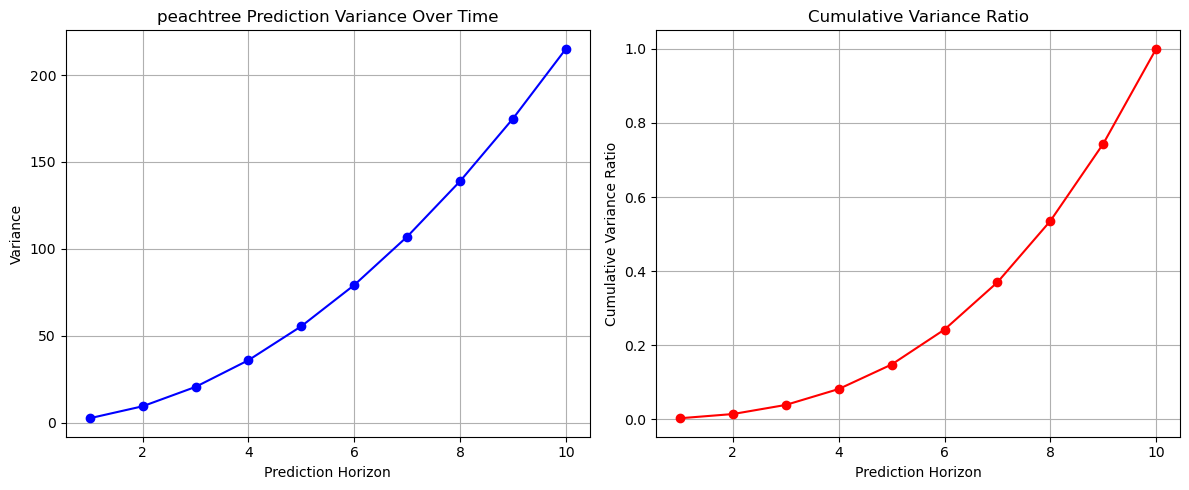
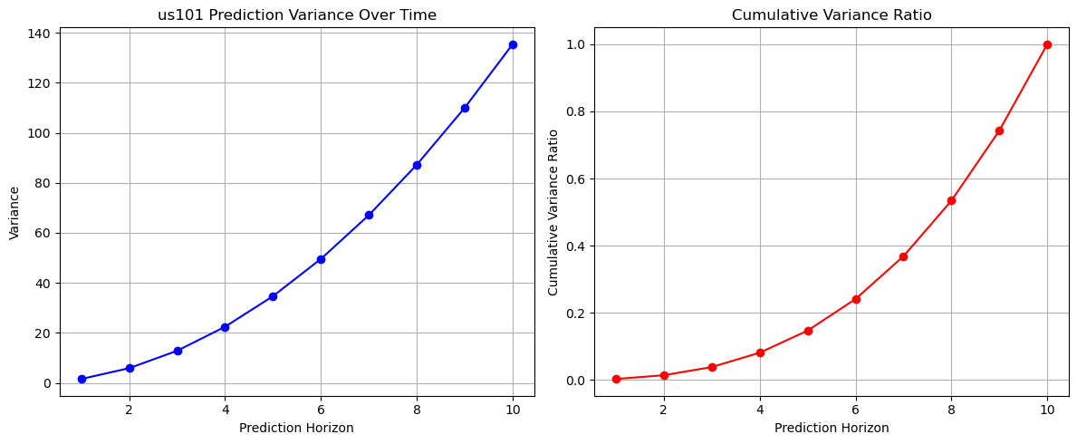
Figure 16: Prediction variance and cumulative variance ratio across datasets
Further variance analysis reveals: I80 shows highest variance (350), followed by Peachtree (200), while US101 demonstrates most stable pattern with variance around 140 at 10-step horizon. Despite different absolute values, their cumulative variance ratios follow similar patterns, suggesting consistent uncertainty accumulation behavior across different traffic environments.
Quantitative Metrics
Evaluation of the models is based on Root Mean Squared Error (RMSE) and Mean Absolute Error (MAE). As we expect a numerical prediction, these metrics show how far the predicted coordinates deviate from the ground truth coordinates. Lower error suggests better performance.
| Linear Regression | LSTM | GMM | |||||||
|---|---|---|---|---|---|---|---|---|---|
| MSE | RMSE | MAE | MSE | RMSE | MAE | MSE | RMSE | MAE | |
| US 101 | 69.95 | 6.09 | 3.78 | 0.8509 | 0.9224 | 0.5944 | 116.31 | 10.78 | 6.87 |
| I80 | 73.58 | 7.12 | 4.60 | 2.1385 | 1.4624 | 0.6320 | 141.32 | 11.89 | 5.96 |
| Peachtree | 87.39 | 7.85 | 4.91 | 27.9767 | 5.2893 | 2.2998 | 103.82 | 10.19 | 5.65 |
LSTM by far outperforms the baselines Linear Regression and GMM. As vehicle trajectory prediction is a complex task that takes into consideration deceleration, interactions with cars and much more, the ability to model sequence in time events is crucial hence LSTM is the best choice. This is exacerbated by road structures such as intersections whereby the behaviour of each vehicle becomes much more complex.
Next Steps
Our project has proposed and evaluated LSTM, Linear Regression and GMM techniques on vehicle trajectory prediction. Next, we will be conducting comparative analysis with advanced deep learning models. Compare the performance of LSTM against other advanced deep learning models such as Transformers, Graph Neural Networks (GNNs). These models may provide additional improvements by better capturing spatial and temporal dependencies.
References
- [1] Afandizadeh S, Sharifi D, Kalantari N, Mirzahossein H. Using machine learning methods to predict electric vehicles penetration in the automotive market. Sci Rep. 2023 May 23;13(1):8345. doi: 10.1038/s41598-023-35366-3. PMID: 37221231; PMCID: PMC10204681.
- [2] H. Jiang, L. Chang, Q. Li and D. Chen, "Trajectory Prediction of Vehicles Based on Deep Learning," 2019 4th International Conference on Intelligent Transportation Engineering (ICITE), Singapore, 2019, pp. 190-195. [Online]. Available: IEEE Explore, doi: 10.1109/ICITE.2019.8880168. [Accessed Oct. 1, 2024].
- [3] L. Lin, W. Li, H. Bi, and L. Qin, "Vehicle trajectory prediction using LSTMs with spatial–temporal attention mechanisms," IEEE Intelligent Transportation Systems Magazine, vol. 14, no. 2, pp. 197-208, Mar.-Apr. 2022. [Online]. Available: IEEE Xplore, doi: 10.1109/MITS.2021.3049404. [Accessed Oct. 1, 2024].
- [4] V. Bharilya and N. Kumar, "Machine learning for autonomous vehicle's trajectory prediction: A comprehensive survey, challenges, and future research directions," Vehicular Communications, vol. 46, Art. no. 100733, 2024. [Online]. Available: ScienceDirect, https://doi.org/10.1016/j.vehcom.2024.100733. [Accessed: Oct. 1, 2024].